Introduction to Power Query with Power BI

Jordan Hohepa, 16 June 2017

This blog is the second in a series of blogs focused on Microsoft’s analytics service, Power BI. In the previous blog I focused on importing data into the Power BI desktop version, while in this blog I will be focusing on Power Query. The data I imported as an example was from the “Rotten Tomatoes Top 100” Web Page and I will continue to use that data in this blog.

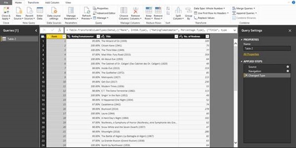
Power Query is a Self-Service ETL (Extract, Transform, Load) tool which is used to ‘transform’ the data imported. Importing data is part of the Power Query step but I decided to cover it on its own in the previous blog. The screenshot above shows the Query Editor window which can be split into four areas:

- The ribbon on top contains buttons which can be used to interact with the table.

- The left pane displays the imported tables.

- The centre pane displays the data of the selected table or selected step

- The right pane shows the Query Settings which contain the properties of the table and the applied steps.

I won’t be going into depth for these areas, but will instead give a quick example using the imported movie data.

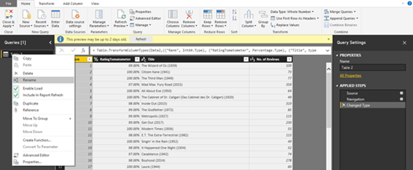
The first thing I noticed with the data was that the Table name wasn’t informative, as the imported table name was “Table 2”. In the screenshot above you can see that by right clicking that table, a set of options are given to edit it. In this example, I will be renaming the table to “Top 100 Movies”.

When interacting with the centre pane we are provided with many different options, allowing us to edit how the data is displayed. Within the table I was given, the 'Ratings' column displayed the values as a percentage in 2 decimal places. As you can see in the screenshot above I could edit this by right clicking the column, going to Change Type and selecting Decimal Number. After this I could rearrange the column order simply by dragging and dropping columns.

The screenshot above now includes the right pane which displays the applied steps. These steps show what transformations will be applied whenever the data is retrieved or refreshed. As you can see it includes the steps we had just done earlier, such as changing the type and reordering the columns.

For the last part of this example I am going to use the Split Column feature which is located in the ribbon under the 'Transform' tab. With the retrieved data, the title column contains both the title of the film and the year it was released which I would like to split into two separate columns. As you can see in the screenshot above I can split a single column into two different columns using a delimiter of my choice. Doing this twice, once for each bracket, allows me to split up the columns and remove the surrounding brackets.

The final screenshot shows the updated table with all the transformation steps applied. Selecting ‘Close & Apply’ in the ribbon will save all these changes and allow us to move onto Power Pivot which will be covered in the next blog.